Histogram based Tomography
Introduction
Quantum states generally encode information about several different mutually incompatible (non-commuting) sets of observables. A given quantum process including final measurement of all qubits will therefore only yield partial information about the pre-measurement state even if the measurement is repeated many times.
To access the information the state contains about other, non-compatible observables, one can apply unitary rotations before measuring. Assuming these rotations are done perfectly, the resulting measurements can be interpreted being of the un-rotated state but with rotated observables.
Quantum tomography is a method that formalizes this procedure and allows to use a complete or overcomplete set of pre-measurement rotations to fully characterize all matrix elements of the density matrix.
Example
Consider a density matrix \(\rho=\begin{pmatrix} 0.3 & 0.2i\\ -0.2i & 0.7\end{pmatrix}\).
Let us assume that our quantum processor’s projective measurement yields perfect outcomes z in the Z basis, either z=+1 or z=-1. Then the density matrix \(\rho\) will give outcome z=+1 with probability p=30% and z=-1 with p=70%, respectively. Consequently, if we repeat the Z-measurement many times, we can estimate the diagonal coefficients of the density matrix. To access the off-diagonals, however, we need to measure different observables such as X or Y.
If we rotate the state as \(\rho\mapsto U\rho U^\dagger\) and then do our usual Z-basis measurement, then this is equivalent to rotating the measured observable as \(Z \mapsto U^\dagger Z U\) and keeping our state \(\rho\) unchanged. This second point of view then allows us to see that if we apply a rotation such as \(U=R_y(\pi/2)\) then this rotates the observable as \(R_y(-\pi/2)ZR_y(+\pi/2)=\cos(\pi/2) Z - \sin(\pi/2) X = -X\). Similarly, we could rotate by \(U=R_x(\pi/2)\) to measure the Y observable. Overall, we can construct a sequence of different circuits with outcome statistics that depend on all elements of the density matrix and that allow to estimate them using techniques such as maximum likelihood estimation ([MLE]).
We have visualized this in Figure 1.
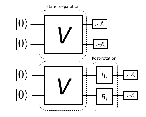
Figure 1: This upper half of this diagram shows a simple 2-qubit quantum program consisting of both qubits initialized in the \(\ket{0}\) state, then transformed to some other state via a process \(V\) and finally measured in the natural qubit basis.
On occasion we may also wish to estimate precisely what physical process a particular control/gate sequence realizes. This is done by a slight extension of the above scheme that also introduces pre-rotations that prepare different initial states, then act on these with the unknown map \(V\) and finally append post-rotations to fully determine the state that each initial state was mapped to. This is visualized in Figure 2.
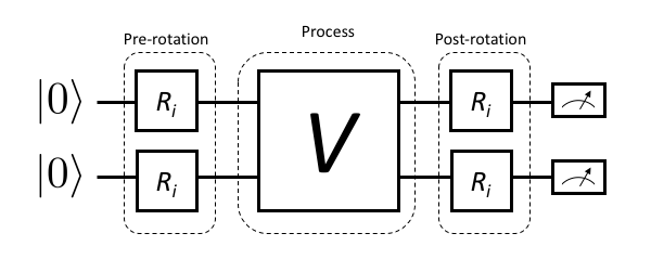
Figure 2: For process tomography, rotations must be prepended and appended to fully resolve the action of V on arbitrary initial states.
The following sections formally define and introduce our tomography methods in full technical detail. Grove also contains an example notebook with tomography results obtained from the QPU. A rendered version of this can be found in example_code.
Useful notation and definitions
In the following we use ‘super-ket’ notation \({\left|\left. \rho \right\rangle\!\right\rangle} := {\text{vec}\left(\hat\rho\right)}\) where \({\text{vec}\left(\hat\rho\right)}\) is a density operator \(\hat\rho\) collapsed to a single vector by stacking its columns. The standard basis in this space is given by \(\{{\left|\left. j \right\rangle\!\right\rangle},\; j=0,1,2\dots, d^2-1\}\), where \(j=f(k,l)\) is a multi-index enumerating the elements of a \(d\)-dimensional matrix row-wise, i.e. \(j=0 \Leftrightarrow (k,l)=(0,0)\), \(j=1 \Leftrightarrow (k,l)=(0,1)\), etc. The super-ket \({\left|\left. j \right\rangle\!\right\rangle}\) then corresponds to the operator \(\ket{k}\bra{l}\).
We similarly define \({\left\langle\!\left\langle \rho \right.\right|} := {\text{vec}\left(\hat\rho\right)}^\dagger\) such that the inner product \({\left\langle\!\left\langle \chi | \rho \right\rangle\!\right\rangle} = {\text{vec}\left(\hat\chi\right)}^\dagger {\text{vec}\left(\hat\rho\right)} = \sum_{j,k=0}^{d^2-1} \chi_{jk}^\ast\rho_{jk} = {\mathrm{Tr}\left(\hat{\chi}^\dagger \hat\rho\right)}\) equals the Hilbert-Schmidt inner product. If \(\rho\) is a physical density matrix and \(\hat{\chi}\) a Hermitian observable, this also equals its expectation value. When a state is represented as a super-ket, we can represent super-operators acting on them as \(\Lambda \to \tilde{\Lambda}\), i.e., we write \({\left|\left. \Lambda(\hat\rho) \right\rangle\!\right\rangle} = \tilde{\Lambda}{\left|\left. \rho \right\rangle\!\right\rangle}\).
We introduce an orthonormal, Hermitian basis for a single qubit in terms of the Pauli operators and the identity \({\left|\left. P_j \right\rangle\!\right\rangle} := {\text{vec}\left(\hat P_j\right)}\) for \(j=0,1,2,3\), where \(\hat P_0 = \mathbb{\hat I}/\sqrt{2}\) and \(\hat P_k=\sigma_{k}/\sqrt{2}\) for \(k=1,2,3\). These satisfy \({\left\langle\!\left\langle P_l | P_m \right\rangle\!\right\rangle}=\delta_{lm}\) for \(l,m=0,1,2,3\). For multi-qubit states, the generalization to a tensor-product basis representation carries over straightforwardly. The normalization \(1/\sqrt{2}\) is generalized to \(1/\sqrt{d}\) for a d-dimensional space. In the following we assume no particular size of the system.
We can then express both states and observables in terms of linear combinations of Pauli-basis super-kets and super-bras, respectively, and they will have real valued coefficients due to the hermiticity of the Pauli operator basis. Starting from an initial state \(\rho\) we can apply a completely positive map to it
A Kraus map is always completely positive and additionally is trace preserving if \(\sum_{j=1}^n \hat K_j^\dagger \hat K_j = \hat I\). We can expand a given map \(\Lambda(\hat\rho)\) in terms of the Pauli basis by exploiting that \(\sum_{j=0}^{d^2-1} {\left|\left. j \right\rangle\!\right\rangle}{\left\langle\!\left\langle j \right.\right|} = \sum_{j=0}^{d^2-1} {\left|\left. \hat P_j \right\rangle\!\right\rangle}{\left\langle\!\left\langle \hat P_j \right.\right|} = \hat{I}\) where \(\hat{I}\) is the super-identity map.
For any given map \(\Lambda(\cdot), \mathcal{B} \rightarrow \mathcal{B}\), where \(\mathcal{B}\) is the space of bounded operators, we can compute its Pauli-transfer matrix as
In contrast to [Chow], our tomography method does not rely on a measurement with continuous outcomes but rather discrete POVM outcomes \(j \in \{0,1,\dots, d-1\}\), where \(d\) is the dimension of the underlying Hilbert space. In the case of perfect readout fidelity the POVM outcome \(j\) coincides with a projective outcome of having measured the basis state \(\ket{j}\). For imperfect measurements, we can falsely register outcomes of type \(k\ne j\) even if the physical state before measurement was \(\ket{j}\). This is quantitatively captured by the readout POVM. Any detection scheme—including the actual readout and subsequent signal processing and classification step to a discrete bitstring outcome—can be characterized by its confusion rate matrix, which provides the conditional probabilities \(p(j|k):= p\)(detected \(j\) \(\mid\) prepared \(k\)) of detected outcome \(j\) given a perfect preparation of basis state \(\ket{k}\)
The trace of the confusion rate matrix ([ConfusionMatrix]) divided by the number of states \(F:={\mathrm{Tr}\left( P\right)}/d = \sum_{j=0}^{d-1} p(j|j)/d\) gives the joint assignment fidelity of our simultaneous qubit readout [Jeffrey], [Magesan]. Given the coefficients appearing in the confusion rate matrix the equivalent readout [POVM] is
where we have introduced the bitstring projectors \(\hat \Pi_{k}=\ket{k}\bra{k}\). We can immediately see that \(\hat N_j\ge 0\) for all \(j\), and verify the normalization
where \(\mathbb{\hat I}\) is the identity operator.
State tomography
For state tomography, we use a control sequence to prepare a state \(\rho\) and then apply \(d^2\) different post-rotations \(\hat R_k\) to our state \(\rho \mapsto \Lambda_{R_k}(\hat \rho) := \hat R_k\hat\rho \hat R_k^\dagger\) such that \({\text{vec}\left(\Lambda_{R_k}(\hat \rho)\right)} = \tilde{\Lambda}_{R_k} {\left|\left. \rho \right\rangle\!\right\rangle}\) and subsequently measure it in our given measurement basis. We assume that subsequent measurements are independent which implies that the relevant statistics for our Maximum-Likelihood-Estimator (MLE) are the histograms of measured POVM outcomes for each prepared state:
If we measure a total of \(n_k = \sum_{j=0}^{d-1} n_{jk}\) shots for the pre-rotation \(\hat R_k\) the probability of obtaining the outcome \(h_k:=(n_{0k}, \dots, n_{(d-1)k})\) is given by the multinomial distribution
where for fixed \(k\) the vector \((p_{0k},\dots, p_{(d-1)k})\) gives the single shot probability over the POVM outcomes for the prepared circuit. These probabilities are given by
Here we have introduced \(\pi_{jl}:={\left\langle\!\left\langle N_j | P_l \right\rangle\!\right\rangle} = {\mathrm{Tr}\left(\hat N_j \hat P_l\right)}\), \((\mathcal{R}_{k})_{rm}:= {\left\langle\!\left\langle P_r \right.\right|}\tilde{\Lambda}_{R_k}{\left|\left. P_m \right\rangle\!\right\rangle}\) and \(\rho_m:= {\left\langle\!\left\langle P_m | \rho \right\rangle\!\right\rangle}\). The POVM operators \(N_j = \sum_{k=0}^{d-1} p(j |k) \Pi_{k}\) are defined as above.
The joint log likelihood for the unknown coefficients \(\rho_m\) for all pre-measurement channels \(\mathcal{R}_k\) is given by
Maximizing this is a convex problem and can be efficiently done even with constraints that enforce normalization \({\mathrm{Tr}\left(\rho\right)}=1\) and positivity \(\rho \ge 0\).
Process Tomography
Process tomography introduces an additional index over the pre-rotations \(\hat R_l\) that act on a fixed initial state \(\rho_0\). The result of each such preparation is then acted on by the process \(\tilde \Lambda\) that is to be inferred. This leads to a sequence of different states
The joint histograms of all such preparations and final POVM outcomes is given by
If we measure a total of \(n_{kl} = \sum_{j=0}^{d-1} n_{jkl}\) shots for the post-rotation \(k\) and pre-rotation \(l,\) the probability of obtaining the outcome \(m_{kl}:=(n_{0kl}, \dots, n_{(d-1)kl})\) is given by the binomial
where the single shot probabilities \(p_{jkl}\) of measuring outcome \(N_j\) for the post-channel \(k\) and pre-channel \(l\) are given by
where \(\pi_{jl}:={\left\langle\!\left\langle N_j | l \right\rangle\!\right\rangle} = {\mathrm{Tr}\left(\hat N_j \hat P_l\right)}\) and \((\rho_0)_q := {\left\langle\!\left\langle P_q | \rho_0 \right\rangle\!\right\rangle} = {\mathrm{Tr}\left(\hat P_q \hat \rho_0\right)}\) and the Pauli-transfer matrices for the pre and post rotations \(R_l\) and the unknown process are given by
The joint log likelihood for the unknown transfer matrix \(\mathcal{R}\) for all pre-rotations \(\mathcal{R}_l\) and post-rotations \(\mathcal{R}_k\) is given by
Handling positivity constraints is achieved by constraining the associated Choi-matrix to be positive [Chow]. We can also constrain the estimated transfer matrix to preserve the trace of the mapped state by demanding that \(\mathcal{R}_{0l}=\delta_{0l}\).
You can learn more about quantum channels here: [QuantumChannel].
Metrics
Here we discuss some quantitative measures of comparing quantum states and processes.
For states
When comparing quantum states there are a variety of different measures of (in-)distinguishability, with each usually being the answer to a particular question, such as “With what probability can I distinguish two states in a single experiment?”, or “How indistinguishable are measurement samples of two states going to be?”.
A particularly easy to compute measure of indistinguishability is given by the quantum state fidelity, which for pure (and normalized) states is simply given by \(F(\phi, \psi)=|\braket{\phi}{\psi}|\). The fidelity is 1 if and only if the two states are identical up to a scalar factor. It is zero when they are orthogonal. The generalization to mixed states takes the form
Although this is not obvious from the expression it is symmetric under exchange of the states. Read more about it here: [QuantumStateFidelity] Although one can use the infidelity \(1-F\) as a distance measure, it is not a proper metric. It can be shown, however that the so called Bures-angle \(\theta _{{\rho \sigma }}\) implicitly defined via \(\cos\theta_{{\rho\sigma}}=F(\rho,\sigma)\) does yield a proper metric in the mathematical sense.
Another useful metric is given by the trace distance ([QuantumTraceDistance])
which is also a proper metric and provides the answer to the above posed question of what the maximum single shot probability is to distinguish states \(\rho\) and \(\sigma\).
For processes
For processes the two most popular metrics are the average gate fidelity \(F_{\rm avg}(P, U)\) of an actual process \(P\) relative to some ideal unitary gate \(U\). In some sense it measures the average fidelity (over all input states) by which a physical channel realizes the ideal operation. Given the Pauli transfer matrices \(\mathcal{R}_P\) and \(\mathcal{R}_U\) for the actual and ideal processes, respectively, the average gate fidelity ([Chow]) is
The corresponding infidelity \(1-F_{\rm avg}(P, U)\) can be seen as a measure of the average gate error, but it is not a proper metric.
Another popular error metric is given by the diamond distance, which is a proper metric and has other nice properties that make it mathematically convenient for proving bounds on error thresholds, etc. It is given by the maximum trace distance between the ideal map and the actual map over all input states \(\rho\) that can generally feature entanglement with other ancillary degrees of freedom that \(U\) acts trivially on.
In a sense, the diamond distance can be seen as a worst case error metric and it is particularly sensitive to coherent gate error, i.e., errors in which P is a (nearly) unitary process but deviates from U. See also these slides by Blume-Kohout et al. for more information [GST].
Further resources
| [MLE] | https://en.wikipedia.org/wiki/Maximum_likelihood_estimation |
| [Chow] | (1, 2, 3) Chow et al. https://doi.org/10.1103/PhysRevLett.109.060501 |
| [Jeffrey] | Jeffrey et al. https://doi.org/10.1103/PhysRevLett.112.190504 |
| [Magesan] | Magesan et al. http://dx.doi.org/10.1103/PhysRevLett.114.200501 |
| [POVM] | https://en.wikipedia.org/wiki/POVM |
| [ConfusionMatrix] | https://en.wikipedia.org/wiki/confusion_matrix |
| [QuantumChannel] | https://en.wikipedia.org/wiki/Quantum_channel |
| [QuantumStateFidelity] | https://en.wikipedia.org/wiki/Fidelity_of_quantum_states |
| [QuantumTraceDistance] | https://en.wikipedia.org/wiki/Trace_distance |
| [GST] | Blume-Kohout et al. https://www.osti.gov/scitech/biblio/1345878 |
Run tomography experiments
This is a rendered version of the example notebook. and provides some example applications of grove’s tomography module.
from __future__ import print_function
import matplotlib.pyplot as plt
from mock import MagicMock
import json

import numpy as np
from grove.tomography.state_tomography import do_state_tomography
from grove.tomography.utils import notebook_mode
from grove.tomography.process_tomography import do_process_tomography

# get fancy TQDM progress bars
notebook_mode(True)

from pyquil.gates import CZ, RY
from pyquil.api import QVMConnection, QPUConnection, get_devices
from pyquil.quil import Program

%matplotlib inline

NUM_SAMPLES = 2000

qvm = QVMConnection()
# QPU
online_devices = [d for d in get_devices() if d.is_online()]
if online_devices:
    d = online_devices[0]
    qpu = QPUConnection(d.name)
    print("Found online device {}, making QPUConnection".format(d.name))
else:
    qpu = QVMConnection()
Found online device 19Q-Acorn, making QPUConnection
Example Code
Create a Bell state
qubits = [6, 7]
bell_state_program = Program(RY(-np.pi/2, qubits[0]),
                             RY(np.pi/2, qubits[1]),
                             CZ(qubits[0],qubits[1]),
                             RY(-np.pi/2, qubits[1]))
Run on QPU & QVM, and calculate the fidelity
%%time
print("Running state tomography on the QPU...")
state_tomography_qpu, _, _ = do_state_tomography(bell_state_program, NUM_SAMPLES, qpu, qubits)
print("State tomography completed.")
print("Running state tomography on the QVM for reference...")
state_tomography_qvm, _, _ = do_state_tomography(bell_state_program, NUM_SAMPLES, qvm, qubits)
print("State tomography completed.")
Running state tomography on the QPU...
State tomography completed.
Running state tomography on the QVM for reference...
State tomography completed.
CPU times: user 1.18 s, sys: 84.2 ms, total: 1.27 s
Wall time: 4.6 s
state_fidelity = state_tomography_qpu.fidelity(state_tomography_qvm.rho_est)
if not SEND_PROGRAMS:
EPS = .01
assert np.isclose(state_fidelity, 1, EPS)
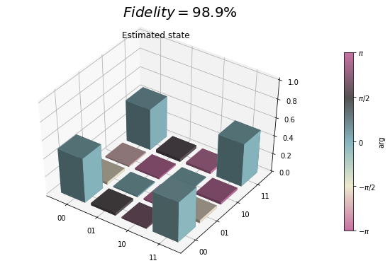
qpu_plot = state_tomography_qpu.plot();
qpu_plot.text(0.35, 0.9, r'$Fidelity={:1.1f}\%$'.format(state_fidelity*100), size=20)
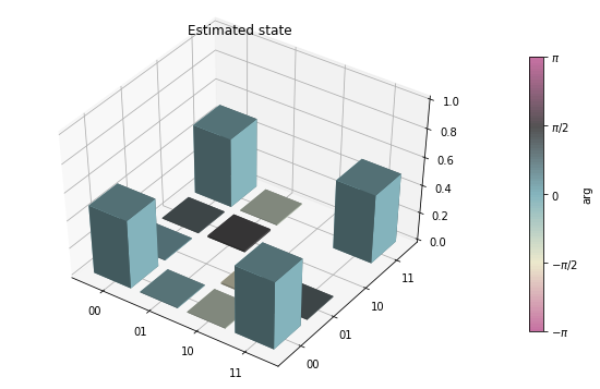
state_tomography_qvm.plot();
Process tomography
Perform process tomography on a controlled-Z (CZ) gate
qubits = [5, 6]
CZ_PROGRAM = Program([CZ(qubits[0], qubits[1])])
print(CZ_PROGRAM)
CZ 5 6
Run on the QPU & QVM, and calculate the fidelity
%%time
print("Running process tomography on the QPU...")
process_tomography_qpu, _, _ = do_process_tomography(CZ_PROGRAM, NUM_SAMPLES, qpu, qubits)
print("Process tomography completed.")
print("Running process tomography on the QVM for reference...")
process_tomography_qvm, _, _ = do_process_tomography(CZ_PROGRAM, NUM_SAMPLES, qvm, qubits)
print("Process tomography completed.")
Running process tomography on the QPU...
Process tomography completed.
Running process tomography on the QVM for reference...
Process tomography completed.
CPU times: user 16.4 s, sys: 491 ms, total: 16.8 s
Wall time: 57.4 s
process_fidelity = process_tomography_qpu.avg_gate_fidelity(process_tomography_qvm.r_est)
if not SEND_PROGRAMS:
EPS = .001
assert np.isclose(process_fidelity, 1, EPS)
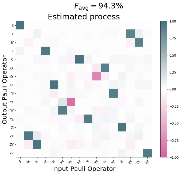
qpu_plot = process_tomography_qpu.plot();
qpu_plot.text(0.4, .95, r'$F_{{\rm avg}}={:1.1f}\%$'.format(process_fidelity*100), size=25)
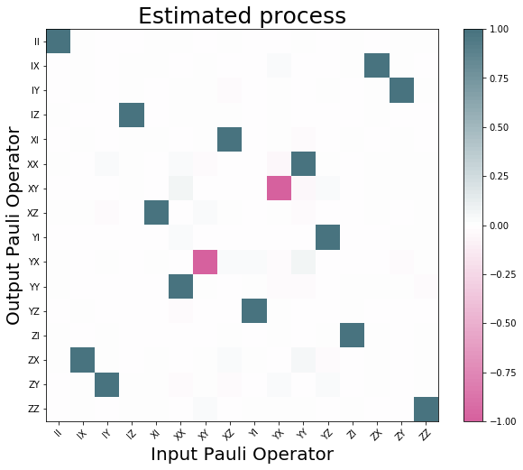
process_tomography_qvm.plot();
Source Code Docs
Module for quantum state and process tomography.
Quantum state and process tomography are algorithms that take as input many copies of a quantum state or process, and output an estimate of what that state or process is. For more information, see the documentation.
-
exception
grove.tomography.tomography.BadReadoutPOVM¶ Bases:
grove.tomography.tomography.TomographyBaseErrorRaised when the tomography analysis fails due to a bad readout calibration.
-
exception
grove.tomography.tomography.IncompleteTomographyError¶ Bases:
grove.tomography.tomography.TomographyBaseErrorRaised when a tomography SignalTensor has circuit results that are all 0. indicating that the measurement did not complete successfully.
-
exception
grove.tomography.tomography.TomographyBaseError¶ Bases:
exceptions.ExceptionBase class for errors raised during Tomography analysis.
-
class
grove.tomography.tomography.TomographySettings¶ Bases:
tupleCreate new instance of TomographySettings(constraints, solver_kwargs)
-
constraints¶ Alias for field number 0
-
solver_kwargs¶ Alias for field number 1
-
-
grove.tomography.tomography.default_channel_ops(nqubits)¶ Generate the tomographic pre- and post-rotations of any number of qubits as qutip operators.
Parameters: nqubits (int) – The number of qubits to perform tomography on. Returns: Qutip object corresponding to the tomographic rotation. Return type: Qobj
-
grove.tomography.tomography.default_rotations(*qubits)¶ Generates the Quil programs for the tomographic pre- and post-rotations of any number of qubits.
Parameters: qubits (list) – A list of qubits to perform tomography on.
-
class
grove.tomography.state_tomography.StateTomography(rho_coeffs, pauli_basis, settings)¶ Bases:
grove.tomography.tomography.TomographyBaseConstruct a StateTomography to encapsulate the result of estimating the quantum state from a quantum tomography measurement.
Parameters: r_est (numpy.ndarray) – The estimated quantum state represented in a given (generalized) Pauli basis. :param OperatorBasis pauli_basis: The employed (generalized) Pauli basis. :param TomographySettings settings: The settings used to estimate the state.
-
static
estimate_from_ssr(histograms, readout_povm, channel_ops, settings)¶ Estimate a density matrix from single shot histograms obtained by measuring bitstrings in the Z-eigenbasis after application of given channel operators.
Parameters: - histograms (numpy.ndarray) – The single shot histograms, shape=(n_channels, dim).
- readout_povm (DiagognalPOVM) – The POVM corresponding to the readout plus classifier.
- channel_ops (list) – The tomography measurement channels as qutip.Qobj’s.
- settings (TomographySettings) – The solver and estimation settings.
Returns: The generated StateTomography object.
Return type:
-
fidelity(other)¶ Compute the quantum state fidelity of the estimated state with another state.
Parameters: other (qutip.Qobj) – The other quantum state. Returns: The fidelity, a real number between 0 and 1. Return type: float
-
plot()¶ Visualize the state.
Returns: The generated figure. Return type: matplotlib.Figure
-
plot_state_histogram(ax)¶ Visualize the complex matrix elements of the estimated state.
Parameters: ax (matplotlib.Axes) – A matplotlib Axes object to plot into.
-
static
-
grove.tomography.state_tomography.do_state_tomography(preparation_program, nsamples, cxn, qubits=None, use_run=False)¶ Method to perform both a QPU and QVM state tomography, and use the latter as as reference to calculate the fidelity of the former.
Parameters: to use in the tomography analysis. :param bool use_run: If
True, use append measurements on all qubits and usecxn.runinstead ofcxn.run_and_measure.Returns: The state tomogram. Return type: StateTomography
-
grove.tomography.state_tomography.state_tomography_programs(state_prep, qubits=None, rotation_generator=<function default_rotations>)¶ Yield tomographic sequences that prepare a state with Quil program state_prep and then append tomographic rotations on the specified qubits. If qubits is None, it assumes all qubits in the program should be tomographically rotated.
Parameters: - state_prep (Program) – The program to prepare the state to be tomographed.
- qubits (list|NoneType) – A list of Qubits or Numbers, to perform the tomography on. If
None, performs it on all in state_prep. :param generator rotation_generator: A generator that yields tomography rotations to perform. :return: Program for state tomography. :rtype: Program
-
class
grove.tomography.process_tomography.ProcessTomography(r_est, pauli_basis, settings)¶ Bases:
grove.tomography.tomography.TomographyBaseConstruct a ProcessTomography to encapsulate the result of estimating a quantum process from a quantum tomography measurement.
Parameters: - r_est (numpy.ndarray) – The estimated quantum process represented as a Pauli transfer matrix.
- pauli_basis (OperatorBasis) – The employed (generalized) Pauli basis.
- settings (TomographySettings) – The settings used to estimate the process.
-
avg_gate_fidelity(reference_unitary)¶ - Compute the average gate fidelity of the estimated process with respect to a unitary
- process. See Chow et al., 2012,
Parameters: reference_unitary ((qutip.Qobj|matrix-like)) – A unitary operator that induces a process as rho -> other*rho*other.dag(), alternatively a superoperator or Pauli-transfer matrix. Returns: The average gate fidelity, a real number between 1/(d+1) and 1, where d is the Hilbert space dimension. :rtype: float
-
static
estimate_from_ssr(histograms, readout_povm, pre_channel_ops, post_channel_ops, settings)¶ Estimate a quantum process from single shot histograms obtained by preparing specific input states and measuring bitstrings in the Z-eigenbasis after application of given channel operators.
Parameters: - histograms (numpy.ndarray) – The single shot histograms.
- readout_povm (DiagonalPOVM) – The POVM corresponding to readout plus classifier.
- pre_channel_ops (list) – The input state preparation channels as qutip.Qobj’s.
- post_channel_ops (list) – The tomography post-process channels as qutip.Qobj’s.
- settings (TomographySettings) – The solver and estimation settings.
Returns: The ProcessTomography object and results from the the given data.
Return type:
-
plot()¶ Visualize the process.
Returns: The generated figure. Return type: matplotlib.Figure
-
plot_pauli_transfer_matrix(ax)¶ Plot the elements of the Pauli transfer matrix.
Parameters: ax (matplotlib.Axes) – A matplotlib Axes object to plot into.
-
process_fidelity(reference_unitary)¶ Compute the quantum process fidelity of the estimated state with respect to a unitary process. For non-sparse reference_unitary, this implementation this will be expensive in higher dimensions.
Parameters: reference_unitary ((qutip.Qobj|matrix-like)) – A unitary operator that induces a process as rho -> other*rho*other.dag(), can also be a superoperator or Pauli-transfer matrix.Returns: The process fidelity, a real number between 0 and 1. Return type: float
-
to_chi()¶ Compute the chi process matrix representation of the estimated process.
Returns: The process as a chi-matrix. Rytpe: qutip.Qobj
-
to_choi()¶ Compute the choi matrix representation of the estimated process.
Returns: The process as a choi-matrix. Rytpe: qutip.Qobj
-
to_kraus()¶ Compute the Kraus operator representation of the estimated process.
Returns: The process as a list of Kraus operators. Rytpe: List[np.array]
-
to_super()¶ Compute the standard superoperator representation of the estimated process.
Returns: The process as a superoperator. Rytpe: qutip.Qobj
-
grove.tomography.process_tomography.do_process_tomography(process, nsamples, cxn, qubits=None, use_run=False)¶ Method to perform a process tomography.
Parameters: to use in the tomography analysis. :param bool use_run: If
True, use append measurements on all qubits and usecxn.runinstead ofcxn.run_and_measure.Returns: The process tomogram Return type: ProcessTomography
-
grove.tomography.process_tomography.process_tomography_programs(process, qubits=None, pre_rotation_generator=<function default_rotations>, post_rotation_generator=<function default_rotations>)¶ Generator that yields tomographic sequences that wrap a process encoded by a QUIL program proc in tomographic rotations on the specified qubits.
If qubits is None, it assumes all qubits in the program should be tomographically rotated.
Parameters: - process (Program) – A Quil program
- qubits (list|NoneType) – The specific qubits for which to generate the tomographic sequences
- pre_rotation_generator – A generator that yields tomographic pre-rotations to perform.
- post_rotation_generator – A generator that yields tomographic post-rotations to perform.
Returns: Program for process tomography.
Return type: Program
-
exception
grove.tomography.operator_utils.CRMBaseError¶ Bases:
exceptions.ExceptionBase class for errors raised when the confusion rate matrix is defective.
-
exception
grove.tomography.operator_utils.CRMUnnormalizedError¶ Bases:
grove.tomography.operator_utils.CRMBaseErrorRaised when a confusion rate matrix is not properly normalized.
-
exception
grove.tomography.operator_utils.CRMValueError¶ Bases:
grove.tomography.operator_utils.CRMBaseErrorRaised when a confusion rate matrix contains elements not contained in the interval :math`[0,1]`
-
class
grove.tomography.operator_utils.DiagonalPOVM¶ Bases:
tupleCreate new instance of DiagonalPOVM(pi_basis, confusion_rate_matrix, ops)
-
confusion_rate_matrix¶ Alias for field number 1
-
ops¶ Alias for field number 2
-
pi_basis¶ Alias for field number 0
-
-
class
grove.tomography.operator_utils.OperatorBasis(labels_ops)¶ Bases:
objectEncapsulates a set of linearly independent operators.
Parameters: labels_ops ((list|tuple)) – Sequence of tuples (label, operator) where label is a string and operator a qutip.Qobj operator representation. -
all_hermitian()¶ Check if all basis operators are hermitian.
-
is_orthonormal()¶ Compute a matrix of Hilbert-Schmidt inner products for the basis operators, and see if they are orthonormal. If they are return True, else, False.
Returns: True if the basis vectors represented by this OperatorBasis are orthonormal, False otherwise. Return type: bool
-
metric()¶ Compute a matrix of Hilbert-Schmidt inner products for the basis operators, update self._metric, and return the value.
Returns: The matrix of inner products. Return type: numpy.matrix
-
product(*bases)¶ Compute the tensor product with another basis.
Parameters: bases – One or more additional bases to form the product with. Return (OperatorBasis): The tensor product basis as an OperatorBasis object.
-
project_op(op)¶ Project an operator onto the basis.
Parameters: op (qutip.Qobj) – The operator to project. Returns: The projection coefficients as a numpy array. Return type: scipy.sparse.csr_matrix
-
super_basis()¶ Generate the superoperator basis in which the Choi matrix can be represented.
The follows the definition in Chow et al.
Return (OperatorBasis): The super basis as an OperatorBasis object.
-
super_from_tm(transfer_matrix)¶ Reconstruct a super operator from a transfer matrix representation. This inverts self.transfer_matrix(…).
Parameters: transfer_matrix ((numpy.ndarray)) – A process in transfer matrix form. Returns: A qutip super operator. Return type: qutip.Qobj.
-
transfer_matrix(superoperator)¶ Compute the transfer matrix \(R_{jk} = r[P_j sop(P_k)]\).
Parameters: superoperator (qutip.Qobj) – The superoperator to transform. Returns: The transfer matrix in sparse form. Return type: scipy.sparse.csr_matrix
-
-
grove.tomography.operator_utils.choi_matrix(pauli_tm, basis)¶ Compute the Choi matrix for a quantum process from its Pauli Transfer Matrix.
This agrees with the definition in Chow et al. except for a different overall normalization. Our normalization agrees with that of qutip.
Parameters: - pauli_tm (numpy.ndarray) – The Pauli Transfer Matrix as 2d-array.
- basis (OperatorBasis) – The operator basis, typically products of normalized Paulis.
Returns: The Choi matrix as qutip.Qobj.
Return type: qutip.Qobj
-
grove.tomography.operator_utils.is_hermitian(operator)¶ Check if matrix or operator is hermitian.
Parameters: operator ((numpy.ndarray|qutip.Qobj)) – The operator or matrix to be tested. Returns: True if the operator is hermitian. Return type: bool
-
grove.tomography.operator_utils.is_projector(operator)¶ Check if operator is a projector.
Parameters: operator (qutip.Qobj) – The operator or matrix to be tested. Returns: True if the operator is a projector. Return type: bool
-
grove.tomography.operator_utils.make_diagonal_povm(pi_basis, confusion_rate_matrix)¶ Create a DiagonalPOVM from a
pi_basisand theconfusion_rate_matrixassociated with a readout.See also the grove documentation.
Parameters: - pi_basis (OperatorBasis) – An operator basis of rank-1 projection operators.
- confusion_rate_matrix (numpy.ndarray) – The matrix of detection probabilities conditional
on a prepared qubit state. :return: The POVM corresponding to confusion_rate_matrix. :rtype: DiagonalPOVM
-
grove.tomography.operator_utils.n_qubit_ground_state(n)¶ Construct the tensor product of n ground states |0>.
Parameters: n (int) – The number of qubits. Returns: The state |000…0> for n qubits. Return type: qutip.Qobj
-
grove.tomography.operator_utils.n_qubit_pauli_basis(n)¶ Construct the tensor product operator basis of n PAULI_BASIS’s.
Parameters: n (int) – The number of qubits. Returns: The product Pauli operator basis of n qubits Return type: OperatorBasis
-
grove.tomography.operator_utils.to_realimag(z)¶ Convert a complex hermitian matrix to a real valued doubled up representation, i.e., for
Z = Z_r + 1j * Z_ireturnR(Z):R(Z) = [ Z_r Z_i] [-Z_i Z_r]
A complex hermitian matrix
Zwith elementwise real and imaginary partsZ = Z_r + 1j * Z_ican be isomorphically represented in doubled up form as:R(Z) = [ Z_r Z_i] [-Z_i Z_r] R(X)*R(Y) = [ (X_r*Y_r-X_i*Y_i) (X_r*Y_i + X_i*Y_r)] [-(X_r*Y_i + X_i*Y_r) (X_r*Y_r-X_i*Y_i) ] = R(X*Y).
In particular,
Zis complex positive (semi-)definite iffR(Z)is real positive (semi-)definite.Parameters: z ((qutip.Qobj|scipy.sparse.base.spmatrix)) – The operator representation matrix. Returns: R(Z) the doubled up representation. Return type: scipy.sparse.csr_matrix
Utilities for encapsulating bases and properties of quantum operators and super-operators as represented by qutip.Qobj()’s.
-
grove.tomography.utils.basis_labels(n)¶ - Generate a list of basis labels for n qubits, ordered from least to greatest, in big-endian
format:
[‘00..00’, ‘00..01’, …, ‘11..11’]
Parameters: n – Returns: A list of strings of length n that enumerate the n-qubit bitstrings Return type: list
-
grove.tomography.utils.basis_state_preps(*qubits)¶ Generate a sequence of programs that prepares the measurement basis states of some set of qubits in the order such that the qubit with highest index is iterated over the most quickly: E.g., for
qubits=(0, 1), it returns the circuits:I_0 I_1 I_0 X_1 X_0 I_1 X_0 X_1
Parameters: qubits (list) – Each qubit to include in the basis state preparation. Returns: Yields programs for each basis state preparation. Return type: Program
-
grove.tomography.utils.bitlist_to_int(bitlist)¶ Convert a binary bitstring into the corresponding unsigned integer.
Parameters: bitlist (list) – A list of ones of zeros. Returns: The corresponding integer. Return type: int
-
grove.tomography.utils.estimate_assignment_probs(bitstring_prep_histograms)¶ Compute the estimated assignment probability matrix for a sequence of single shot histograms obtained by running the programs generated by basis_state_preps().
bitstring_prep_histograms[i,j] = #number of measured outcomes j when running program iThe assignment probability is obtained by transposing and afterwards normalizing the columns.
p[j, i] = Probability to measure outcome j when preparing the state with program i.Parameters: bitstring_prep_histograms (list|numpy.ndarray) – A nested list or 2d array with shape (d, d), where
d = 2**nqubitsis the dimension of the Hilbert space. The first axis varies over the state preparation program index, the second axis corresponds to the measured bitstring. :return: The assignment probability matrix. :rtype: numpy.ndarray
-
grove.tomography.utils.generated_states(initial_state, preparations)¶ Generate states prepared from channel operators acting on an initial state. Typically the channel operators will be unitary.
Parameters: - initial_state (qutip.Qobj) – The initial state as a density matrix.
- preparations ((list|tuple)) – The unitary channel operators that transform the initial state.
Returns: The states generated from preparations acting on intial_state
Return type:
-
grove.tomography.utils.import_cvxpy()¶ Try importing the qutip module, log an error if unsuccessful.
Returns: The cvxpy module if successful or None Return type: Optional[module]
-
grove.tomography.utils.import_qutip()¶ Try importing the qutip module, log an error if unsuccessful.
Returns: The qutip module if successful or None Return type: Optional[module]
-
grove.tomography.utils.make_histogram(samples, ksup)¶ For a list of samples [s1, s2, …, sN] taking on integer values from 0 to ksup-1, make a histogram of each integer’s outcome and return it.
Parameters: - samples – The samples.
- ksup – The (exclusive) upper bound
Returns: A histogram of outcomes.
Return type: numpy.ndarray
-
grove.tomography.utils.notebook_mode(m)¶ Configure whether this module should assume that it is being run from a jupyter notebook. This sets some global variables related to how progress for long measurement sequences is indicated.
Parameters: m (bool) – If True, assume to be in notebook. Returns: None Return type: NoneType
-
grove.tomography.utils.plot_pauli_transfer_matrix(ptransfermatrix, ax, labels, title)¶ Visualize the Pauli Transfer Matrix of a process.
Parameters: - ptransfermatrix (numpy.ndarray) – The Pauli Transfer Matrix
- ax – The matplotlib axes.
- labels – The labels for the operator basis states.
- title – The title for the plot
Returns: The modified axis object.
Return type: AxesSubplot
-
grove.tomography.utils.run_in_parallel(programs, nsamples, cxn, shuffle=True)¶ Take sequences of Protoquil programs on disjoint qubits and execute a single sequence of programs that executes the input programs in parallel. Optionally randomize within each qubit-specific sequence.
The programs are passed as a 2d array of Quil programs, where the (first) outer axis iterates over disjoint sets of qubits that the programs involve and the inner axis iterates over a sequence of related programs, e.g., tomography sequences, on the same set of qubits.
Parameters: - programs (Union[np.ndarray,List[List[Program]]]) – A rectangular list of lists, or a 2d array of Quil Programs. The outer list iterates over disjoint qubit groups as targets, the inner list over programs to run on those qubits, e.g., tomographic sequences.
- nsamples (int) – Number of repetitions for executing each Program.
- cxn (QPUConnection|QVMConnection) – The quantum machine connection.
- shuffle (bool) – If True, the order of each qubit specific sequence (2nd axis) is randomized Default is True.
Returns: An array of 2d arrays that provide bitstring histograms for each input program. The axis of the outer array iterates over the disjoint qubit groups, the outer axis of the inner 2d array iterates over the programs for that group and the inner most axis iterates over all possible bitstrings for the qubit group under consideration.
:rtype np.array
-
grove.tomography.utils.sample_assignment_probs(qubits, nsamples, cxn)¶ Sample the assignment probabilities of qubits using nsamples per measurement, and then compute the estimated assignment probability matrix. See the docstring for estimate_assignment_probs for more information.
Parameters: Returns: The assignment probability matrix.
Return type: numpy.ndarray
-
grove.tomography.utils.sample_bad_readout(program, num_samples, assignment_probs, cxn)¶ Generate n samples of measuring all outcomes of a Quil program assuming the assignment probabilities assignment_probs by simulating the wave function on a qvm QVMConnection cxn
Parameters: - program (pyquil.quil.Program) – The program.
- num_samples (int) – The number of samples
- assignment_probs (numpy.ndarray) – A matrix of assignment probabilities
- cxn (QVMConnection) – the QVM connection.
Returns: The resulting sampled outcomes from assignment_probs applied to cxn, one dimensional.
Return type: numpy.ndarray
-
grove.tomography.utils.sample_outcomes(probs, n)¶ For a discrete probability distribution
probswith outcomes 0, 1, …, k-1 drawnrandom samples.Parameters: - probs (list) – A list of probabilities.
- n (Number) – The number of random samples to draw.
Returns: An array of samples drawn from distribution probs over 0, …, len(probs) - 1
Return type: numpy.ndarray
-
grove.tomography.utils.state_histogram(rho, ax=None, title='', threshold=0.001)¶ Visualize a density matrix as a 3d bar plot with complex phase encoded as the bar color.
This code is a modified version of an equivalent function in qutip which is released under the (New) BSD license.
Parameters: are hidden. :return: The axis :rtype: mpl_toolkits.mplot3d.Axes3D
-
grove.tomography.utils.to_density_matrix(state)¶ Convert a Hilbert space vector to a density matrix.
Parameters: state (qt.basis) – The state to convert into a density matrix. Returns: The density operator corresponding to state. Return type: qutip.qobj.Qobj