Variational-Quantum-Eigensolver (VQE)
Overview
The Variational-Quantum-Eigensolver (VQE) [1, 2] is a quantum/classical hybrid algorithm that can be used to find eigenvalues of a (often large) matrix \(H\). When this algorithm is used in quantum simulations, \(H\) is typically the Hamiltonian of some system [3, 4, 5]. In this hybrid algorithm a quantum subroutine is run inside of a classical optimization loop.
The quantum subroutine has two fundamental steps:
- Prepare the quantum state \(|\Psi(\vec{\theta})\rangle\), often called the ansatz.
- Measure the expectation value \(\langle\,\Psi(\vec{\theta})\,|\,H\,|\,\Psi(\vec{\theta})\,\rangle\).
The variational principle ensures that this expectation value is always greater than the smallest eigenvalue of \(H\).
This bound allows us to use classical computation to run an optimization loop to find this eigenvalue:
- Use a classical non-linear optimizer to minimize the expectation value by varying ansatz parameters \(\vec{\theta}\).
- Iterate until convergence.
Practically, the quantum subroutine of VQE amounts to preparing a state based off
of a set of parameters \(\vec{\theta}\) and performing a series of measurements
in the appropriate basis. The paramaterized state (or ansatz) preparation can be tricky
in these algorithms and can dramatically affect performance. Our VQE module allows any
Python function that returns a pyQuil program to be used as an ansatz generator. This
function is passed into vqe_run as the variational_state_evolve argument. More details
are in the source documentation.
Measurements are then performed on these states based on a Pauli operator decomposition of \(H\). Using Quil, these measurements will end up in classical memory. Doing this iteratively followed by a small amount of postprocessing, one may compute a real expectation value for the classical optimizer to use.
Below there is a very small first example of VQE and Grove’s implementation of the Quantum Approximate Optimization Algorithm QAOA also makes use of the VQE module.
Basic Usage
Here we will take you through an example of a very small variational quantum eigensolver problem. In this example we will use a quantum circuit that consists of a single parametrized gate to calculate an eigenvalue of the Pauli Z matrix.
First we import the necessary pyQuil modules to construct our ansatz pyQuil program.
from pyquil.quil import Program
import pyquil.api as api
from pyquil.gates import *
qvm = api.QVMConnection()
Any Python function that takes a list of numeric parameters and outputs a pyQuil program can be used as an ansatz function. We will see some more examples of this later. For now, we just take a parameter list with a single parameter.
def small_ansatz(params):
    return Program(RX(params[0], 0))

print(small_ansatz([1.0]))
RX(1.0) 0
This small_ansatz function is our \(\Psi(\vec{\theta})\). To
construct the Hamiltonian that we wish to simulate, we use the
pyquil.paulis module.
from pyquil.paulis import sZ
initial_angle = [0.0]
# Our Hamiltonian is just \sigma_z on the zeroth qubit
hamiltonian = sZ(0)
We now use the vqe module in Grove to construct a VQE object to perform
our algorithm. In this example, we use scipy.optimize.minimize()
with Nelder-Mead as our classical minimizer, but you can choose other
parameters or write your own minimizer.
from grove.pyvqe.vqe import VQE
from scipy.optimize import minimize
import numpy as np

vqe_inst = VQE(minimizer=minimize,
               minimizer_kwargs={'method': 'nelder-mead'})
Before we run the minimizer, let us look manually at what expectation values \(\langle\,\Psi(\vec{\theta})\,|\,H\,|\,\Psi(\vec{\theta})\,\rangle\) we calculate for fixed parameters of \(\vec{\theta}\).
angle = 2.0
vqe_inst.expectation(small_ansatz([angle]), hamiltonian, None, qvm)
-0.4161468365471423
The expectation value was calculated by running the pyQuil program output from
small_ansatz, saving the wavefunction, and using that vector to calculate
the expectation value. We can sample the wavefunction as you would on a
quantum computer by passing an integer, instead of None, as the samples
argument of the expectation() method.
angle = 2.0
vqe_inst.expectation(small_ansatz([angle]), hamiltonian, 10000, qvm)
-0.42900000000000005
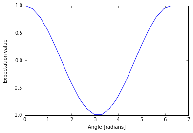
We can loop over a range of these angles and plot the expectation value.
angle_range = np.linspace(0.0, 2 * np.pi, 20)
data = [vqe_inst.expectation(small_ansatz([angle]), hamiltonian, None, qvm)
        for angle in angle_range]

import matplotlib.pyplot as plt
plt.xlabel('Angle [radians]')
plt.ylabel('Expectation value')
plt.plot(angle_range, data)
plt.show()
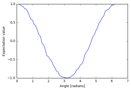
Now with sampling…
angle_range = np.linspace(0.0, 2 * np.pi, 20)
data = [vqe_inst.expectation(small_ansatz([angle]), hamiltonian, 1000, qvm)
        for angle in angle_range]

import matplotlib.pyplot as plt
plt.xlabel('Angle [radians]')
plt.ylabel('Expectation value')
plt.plot(angle_range, data)
plt.show()
We can compare this plot against the value we obtain when we run the our variational quantum eigensolver.
result = vqe_inst.vqe_run(small_ansatz, hamiltonian, initial_angle, None, qvm=qvm)
print(result)
{'fun': -0.99999999954538055, 'x': array([ 3.1415625])}
Running Noisy VQE
A great thing about VQE is that it is somewhat insensitive to noise. We can test this out by running the previous algorithm on a noisy qvm.
Remember that Pauli channels are defined as a list of three probabilities that correspond to the probability of a random X, Y, or Z gate respectively. First we’ll study the impact of a channel that has the same probability of each random Pauli.
pauli_channel = [0.1, 0.1, 0.1] #10% chance of each gate at each timestep
noisy_qvm = api.QVMConnection(gate_noise=pauli_channel)
Let us check that this QVM has noise:
p = Program(X(0), X(1)).measure(0, [0]).measure(1, [1])
noisy_qvm.run(p, [0, 1], 10)
[[1, 1],
 [0, 1],
 [1, 0],
 [0, 1],
 [0, 0],
 [1, 1],
 [0, 1],
 [1, 0],
 [1, 0],
 [0, 1]]
We can run the VQE under noise. Let’s modify the classical optimizer to start with a larger simplex so we don’t get stuck at an initial minimum.
vqe_inst.minimizer_kwargs = {'method': 'Nelder-mead', 'options': {'initial_simplex': np.array([[0.0], [0.05]]), 'xatol': 1.0e-2}}
result = vqe_inst.vqe_run(small_ansatz, hamiltonian, initial_angle, samples=10000, qvm=noisy_qvm)
print(result)
{'fun': 0.5875999999999999, 'x': array([ 0.01874886])}
10% error is a huge amount of error! We can plot the effect of increasing noise on the result of this algorithm:
data = []
noises = np.linspace(0.0, 0.01, 4)
for noise in noises:
    pauli_channel = [noise] * 3
    noisy_qvm = api.QVMConnection(gate_noise=pauli_channel)
    # We can pass the noise params directly into the vqe_run instead of passing the noisy connection
    result = vqe_inst.vqe_run(small_ansatz, hamiltonian, initial_angle,
                          gate_noise=pauli_channel)
    data.append(result['fun'])
plt.xlabel('Noise level %')
plt.ylabel('Eigenvalue')
plt.plot(noises, data)
plt.show()
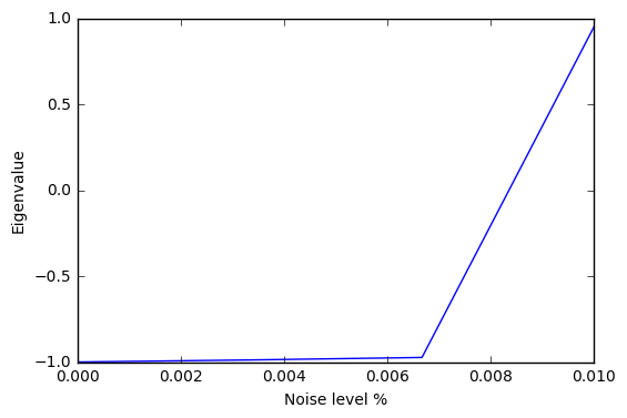
It looks like this algorithm is pretty robust to noise up until 0.6% error. However measurement noise might be a different story.
meas_channel = [0.1, 0.1, 0.1] #10% chance of each gate at each measurement
noisy_meas_qvm = api.QVMConnection(measurement_noise=meas_channel)
Measurement noise has a different effect:
p = Program(X(0), X(1)).measure(0, [0]).measure(1, [1])
noisy_meas_qvm.run(p, [0, 1], 10)
[[1, 1],
 [1, 1],
 [1, 1],
 [1, 1],
 [1, 1],
 [1, 1],
 [0, 1],
 [1, 0],
 [1, 1],
 [1, 0]]
data = []
noises = np.linspace(0.0, 0.01, 4)
for noise in noises:
    meas_channel = [noise] * 3
    noisy_qvm = api.QVMConnection(measurement_noise=meas_channel)
    result = vqe_inst.vqe_run(small_ansatz, hamiltonian, initial_angle, samples=10000, qvm=noisy_qvm)
    data.append(result['fun'])
plt.xlabel('Noise level %')
plt.ylabel('Eigenvalue')
plt.plot(noises, data)
plt.show()
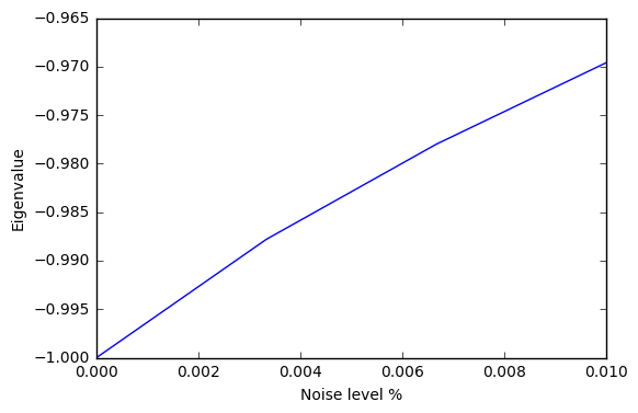
We see this particular VQE algorithm is generally more sensitive to measurement noise than gate noise.
More Sophisticated Ansatzes
Because we are working with Python, we can leverage the full language to make much more sophisticated ansatzes for VQE. As an example we can easily change the number of gates.
def smallish_ansatz(params):
    return Program(RX(params[0], 0), RX(params[1], 0))

print(smallish_ansatz([1.0, 2.0]))
RX(1.0) 0
RX(2.0) 0
vqe_inst = VQE(minimizer=minimize,
               minimizer_kwargs={'method': 'nelder-mead'})
initial_angles = [1.0, 1.0]
result = vqe_inst.vqe_run(smallish_ansatz, hamiltonian, initial_angles, None, qvm=qvm)
print(result)
{'fun': -1.0000000000000004, 'x': array([ 1.61767133, 1.52392133])}
We can even dynamically change the gates in the circuit based on a parameterization:
def variable_gate_ansatz(params):
    gate_num = int(np.round(params[1])) # for scipy.minimize params must be floats
    p = Program(RX(params[0], 0))
    for gate in range(gate_num):
        p.inst(X(0))
    return p

print(variable_gate_ansatz([0.5, 3]))
RX(0.5) 0
X 0
X 0
X 0
initial_params = [1.0, 3]
result = vqe_inst.vqe_run(variable_gate_ansatz, hamiltonian, initial_params, None, qvm=qvm)
print(result)
{'fun': -1.0, 'x': array([ 2.65393312e-09, 3.42891875e+00])}
Note that the restriction that the ansatz function take a single list of
floats as parameters only comes from our choice of minimizer (this is
what scipy.optimize.minimize takes). One could easily imagine
writing a custom minimizer that takes more sophisticated forms of
arguments.
Links and Further Reading
This concludes our brief tour of VQE. There is a lot of fascinating literature about this algorithm out there and we encourage you to both explore those topics as well as come up with new ideas using this library. Let us know if you have ideas about anything that you would like to see added!
Here are some links to get you started:
- A Variational Eigenvalue Solver on a Quantum Processor
- The Theory of Variational Hybrid Quantum-Classical Algorithms
- Hybrid Quantum-Classical Approach to Correlated Materials
- A Hybrid Classical/Quantum Approach for Large-Scale Studies of Quantum Systems with Density Matrix Embedding Theory
- Hybrid Quantum-Classical Hierarchy for Mitigation of Decoherence and Determination of Excited States
Source Code Docs
Here you can find documentation for the different submodules in pyVQE.
grove.pyvqe.vqe
-
class
grove.pyvqe.vqe.VQE(minimizer, minimizer_args=[], minimizer_kwargs={})¶ Bases:
objectThe Variational-Quantum-Eigensolver algorithm
VQE is an object that encapsulates the VQE algorithm (functional minimization). The main components of the VQE algorithm are a minimizer function for performing the functional minimization, a function that takes a vector of parameters and returns a pyQuil program, and a Hamiltonian of which to calculate the expectation value.
Using this object:
1) initialize with inst = VQE(minimizer) where minimizer is a function that performs a gradient free minization–i.e scipy.optimize.minimize(. , ., method=’Nelder-Mead’)
2) call inst.vqe_run(variational_state_evolve, hamiltonian, initial_parameters). Returns the optimal parameters and minimum expecation
Parameters: - minimizer – function that minimizes objective f(obj, param). For example the function scipy.optimize.minimize() needs at least two parameters, the objective and an initial point for the optimization. The args for minimizer are the cost function (provided by this class), initial parameters (passed to vqe_run() method, and jacobian (defaulted to None). kwargs can be passed in below.
- minimizer_args – (list) arguments for minimizer function. Default=None
- minimizer_kwargs – (dict) arguments for keyword args. Default=None
-
static
expectation(pyquil_prog, pauli_sum, samples, qvm)¶ Computes the expectation value of pauli_sum over the distribution generated from pyquil_prog.
Parameters: - pyquil_prog – (pyQuil program)
- pauli_sum – (PauliSum, ndarray) PauliSum representing the operator of which to calculate the expectation value or a numpy matrix representing the Hamiltonian tensored up to the appropriate size.
- samples – (int) number of samples used to calculate the expectation value. If samples is None then the expectation value is calculated by calculating <psi|O|psi> on the QVM. Error models will not work if samples is None.
- qvm – (qvm connection)
Returns: (float) representing the expectation value of pauli_sum given given the distribution generated from quil_prog.
-
vqe_run(variational_state_evolve, hamiltonian, initial_params, gate_noise=None, measurement_noise=None, jacobian=None, qvm=None, disp=None, samples=None, return_all=False)¶ functional minimization loop.
Parameters: - variational_state_evolve – function that takes a set of parameters and returns a pyQuil program.
- hamiltonian – (PauliSum) object representing the hamiltonian of which to take the expectation value.
- initial_params – (ndarray) vector of initial parameters for the optimization
- gate_noise – list of Px, Py, Pz probabilities of gate being applied to every gate after each get application
- measurement_noise – list of Px’, Py’, Pz’ probabilities of a X, Y or Z being applied before a measurement.
- jacobian – (optional) method of generating jacobian for parameters (Default=None).
- qvm – (optional, QVM) forest connection object.
- disp – (optional, bool) display level. If True then each iteration expectation and parameters are printed at each optimization iteration.
- samples – (int) Number of samples for calculating the expectation value of the operators. If None then faster method ,dotting the wave function with the operator, is used. Default=None.
- return_all – (optional, bool) request to return all intermediate parameters determined during the optimization.
Returns: (vqe.OptResult()) object
OptResult. The following fields are initialized in OptResult: -x: set of w.f. ansatz parameters -fun: scalar value of the objective function- -iteration_params: a list of all intermediate parameter vectors. Only
returned if ‘return_all=True’ is set as a vqe_run() option.
- -expectation_vals: a list of all intermediate expectation values. Only
returned if ‘return_all=True’ is set as a vqe_run() option.
-
grove.pyvqe.vqe.expectation_from_sampling(pyquil_program, marked_qubits, qvm, samples)¶ Calculation of Z_{i} at marked_qubits
Given a wavefunctions, this calculates the expectation value of the Zi operator where i ranges over all the qubits given in marked_qubits.
Parameters: - pyquil_program – pyQuil program generating some state
- marked_qubits – The qubits within the support of the Z pauli operator whose expectation value is being calculated
- qvm – A QVM connection.
- samples – Number of bitstrings collected to calculate expectation from sampling.
Returns: The expectation value as a float.
-
grove.pyvqe.vqe.parity_even_p(state, marked_qubits)¶ Calculates the parity of elements at indexes in marked_qubits
Parity is relative to the binary representation of the integer state.
Parameters: - state – The wavefunction index that corresponds to this state.
- marked_qubits – The indexes to be considered in the parity sum.
Returns: A boolean corresponding to the parity.