Quantum Approximate Optimization Algorithm (QAOA)
Overview
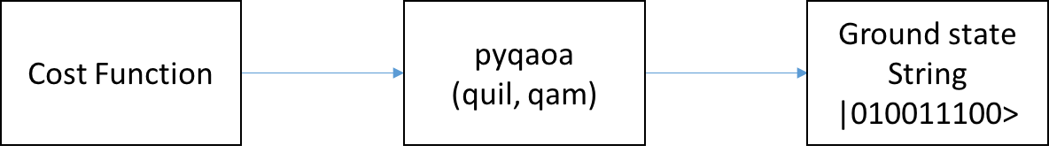
pyQAOA is a Python module for running the Quantum Approximate Optimization Algorithm on an instance of a quantum abstract machine.
The pyQAOA package contains separate modules for each type of problem instance: MAX-CUT, graph partitioning, etc. For each problem instance the user specifies the driver Hamiltonian, cost Hamiltonian, and the approximation order of the algorithm.
qaoa.py contains the base QAOA class and routines for finding optimal
rotation angles via Grove’s
variational-quantum-eigensolver method.
Cost Functions
maxcut_qaoa.pyimplements the cost function for MAX-CUT problems.numpartition_qaoa.pyimplements the cost function for bipartitioning a list of numbers.
Quickstart Examples
To test your installation and get going we can run QAOA to solve MAX-CUT on a square ring with 4 nodes at the corners. In your python interpreter import the packages and connect to your QVM:
import numpy as np
from grove.pyqaoa.maxcut_qaoa import maxcut_qaoa
import pyquil.api as api
qvm_connection = api.QVMConnection()
Next define the graph on which to run MAX-CUT
square_ring = [(0,1),(1,2),(2,3),(3,0)]
The optional configuration parameter for the algorithm is given by the number of steps to use (which loosely corresponds to the accuracy of the optimization computation). We instantiate the algorithm and run the optimization routine on our QVM:
steps = 2
inst = maxcut_qaoa(graph=square_ring, steps=steps)
betas, gammas = inst.get_angles()
to see the final \(\mid \beta, \gamma \rangle \) state we can rebuild the quil program that gives us \(\mid \beta, \gamma \rangle \) and evaluate the wave function using the QVM
t = np.hstack((betas, gammas))
param_prog = inst.get_parameterized_program()
prog = param_prog(t)
wf = qvm_connection.wavefunction(prog)
wf = wf.amplitudes
wf is now a numpy array of complex-valued amplitudes for each computational
basis state. To visualize the distribution iterate over the states and
calculate the probability.
for state_index in range(inst.nstates):
    print(inst.states[state_index], np.conj(wf[state_index])*wf[state_index])
You should then see that the algorithm converges on the expected solutions of 0101 and 1010!
0000 (4.38395094039e-26+0j)
0001 (5.26193287055e-15+0j)
0010 (5.2619328789e-15+0j)
0011 (1.52416449345e-13+0j)
0100 (5.26193285935e-15+0j)
0101 (0.5+0j)
0110 (1.52416449362e-13+0j)
0111 (5.26193286607e-15+0j)
1000 (5.26193286607e-15+0j)
1001 (1.52416449362e-13+0j)
1010 (0.5+0j)
1011 (5.26193285935e-15+0j)
1100 (1.52416449345e-13+0j)
1101 (5.2619328789e-15+0j)
1110 (5.26193287055e-15+0j)
1111 (4.38395094039e-26+0j)
Algorithm and Details
Introduction
The quantum-approximate-optimization-algorithm (QAOA, pronouced quah-wah), developed by Farhi, Goldstone, and Gutmann, is a polynomial time algorithm for finding “a ‘good’ solution to an optimization problem” [1, 2].
What’s with the name? For a given NP-Hard problem an approximate algorithm is a polynomial-time algorithm that solves every instance of the problem with some guaranteed quality in expectation. The value of merit is the ratio between the quality of the polynomial time solution and the quality of the true solution.
One reason QAOA is interesting is its potential to exhibit quantum supremacy [1].
This package, which is an implementation of QAOA that runs on a simulated quantum computer, can be used as a stand alone optimizer or a plugin optimization routine in a larger environment. The usage pipeline is as follows: 1) encoding the cost function into a set of Pauli operators, 2) instantiating the problem with pyQAOA and pyQuil, and 3) retrieving ground state solution by sampling.
The following section of the pyQAOA documentation describes the algorithm and the NP-hard problem instance used in the original paper.
Our First NP-Hard Problem
The maximum-cut problem (MAX-CUT) was the first application described in the original quantum-approximate-optimization-algorithm paper [2 ]. This problem is similar to graph coloring. Given a graph of nodes and edges, color each node black or white, then score a point for each node that is next to a node of a different color. The aim is to find a coloring that scores the most points.
Stated a bit more formally, the problem is to partition the nodes of a graph into two sets such that the number of edges connecting nodes in opposite sets is maximized. For example, consider the barbell graph
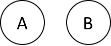
there are 4 ways of partitioning nodes into two sets:
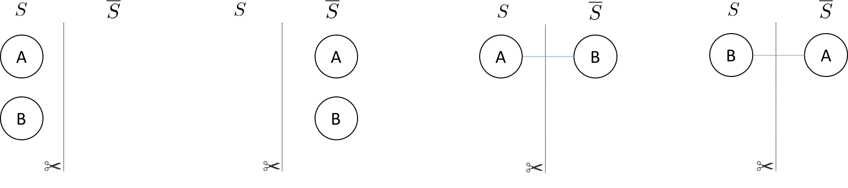
We have drawn the edge only when it connects nodes in different sets. The line with the scissor symbol indicates that we count the edge in our cut. For the barbell graph there are two equal weight partitionings that correspond to a maximum cut (the right two partitonings)–i.e. cutting the barbell in half. One can denote which set \( S \) or \( \overline{S} \) a node is in with either a \(0\) or a \(1\), respectively, in a bit string of length \( N \). The four partitionings of the barbell graph listed above are, \(\{ 00, 11, 01, 10 \} \)—where the left most bit is node \(A\) and the right most bit is node \(B\). The bit string representation makes it easy to represent a particular partition of the graph. Each bit string has an associated cut weight.
For any graph, the bit string representations of the node partitionings are always length \(N\). The total number of partitionings grows as \(2^{N}\). For example, a square ring graph
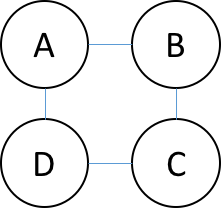
has 16 possible partitions (\(2^{4}\)). Below are two possible ways of parititioning of the nodes.
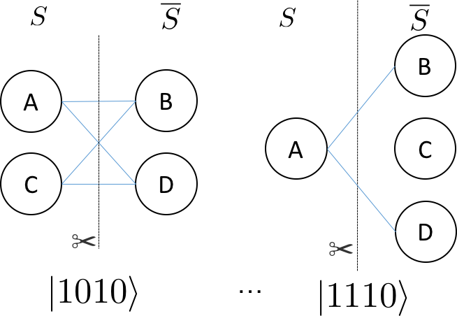
The bit strings associated with each parititioning are indicated in the figure. The right most bit corresponds with the node labeled \(A\) and the left most bit corresponds with the node labeled \(D\).
Classical Solutions
In order to find the best cut on a classical computer the obvious approach is to enumerate all partitions of the graph and check the weight of the cut associated with the partition.
Faced with an exponential cost for finding the optimal cut (or set of optimal cuts) one can devise a polynomial algorithm that is guaranteed to be of a particular quality. For example, a famous polynomial time algorithm is the randomized partitioning approach. One simply iterates over the nodes of the graph and flips a coin. If the coin is heads the node is in \( S \), if tails the node is in \( \overline{S} \). The quality of the random assignment algorithm is at least 50 percent of the maximum cut. For a coin-flip process the probability of an edge being in the cut is 50%. Therefore, the expectation value of a cut produced by random assignment can be written as follows: $$\sum_{e \in E} w_{e} \cdot \mathrm{Pr}(e \in \mathrm{cut}) = \frac{1}{2} \sum_{e \in E}w_{e}$$ Since the sum of all the edges is necessarily an upper bound to the maximum cut the randomized approach produces a cut of expected value of at least 0.5 times the best cut on the graph.
Other polynomial approaches exist that involve semi-definite programming which give cuts of expected value at least 0.87856 times the maximum cut [3].
Quantum Approximate Optimization
One can think of the bit strings (or set of bit strings) that correspond to the maximum cut on a graph as the ground state of a Hamiltonian encoding the cost function. The form of this Hamiltonian can be determined by constructing the classical function that returns a 1 (or the weight of the edge) if the edge spans two-nodes in different sets, or 0 if the nodes are in the same set. \begin{align} C_{ij} = \frac{1}{2}(1 - z_{i}z_{j}) \end{align} \( z_{i}\) or \(z_{j}\) is \(+1\) if node \(i\) or node \(j\) is in \(S\) or \(-1\) if node \(i\) or node \(j\) is in \(\overline{S}\). The total cost is the sum of all \( (i ,j) \) node pairs that form the edge set of the graph. This suggests that for MAX-CUT the Hamiltonian that encodes the problem is $$\sum_{ij}\frac{1}{2}(\mathbf{I} - \sigma_{i}^{z}\sigma_{j}^{z})$$ where the sum is over \( (i,j) \) node pairs that form the edges of the graph. The quantum-approximate-optimization-algorithm relies on the fact that we can prepare something approximating the ground state of this Hamiltonian and perform a measurement on that state. Performing a measurement on the \(N\)-body quantum state returns the bit string corresponding to the maximum cut with high probability.
To make this concrete let us return to the barbell graph. The graph requires two qubits in order to represent the nodes. The Hamiltonian has the form \begin{align} \hat{H} = \frac{1}{2}(\mathbf{I} - \sigma_{z}^{1}\otimes \sigma_{z}^{0}) = \begin{pmatrix} 0 & 0 & 0 & 0 \ 0 & 1 & 0 & 0 \ 0 & 0 & 1 & 0 \ 0 & 0 & 0 & 0 \end{pmatrix} \end{align} where the basis ordering corresponds to increasing integer values in binary format (the left most bit being the most significant). This corresponds to a basis ordering for the \(\hat{H}\) operator above as \begin{align} (| 00\rangle, | 01\rangle, | 10\rangle, | 11\rangle). \end{align} Here the Hamiltonian is diagonal with integer eigenvalues. Clearly each bit string is an eigenstate of the Hamiltonian because \(\hat{H}\) is diagonal.
QAOA identifies the ground state of the MAXCUT Hamiltonian by evolving from a reference state. This reference state is the ground state of a Hamiltonian that couples all \( 2^{N} \) states that form the basis of the cost Hamiltonian—i.e. the diagonal basis for cost function. For MAX-CUT this is the \(Z\) computational basis.
The evolution between the ground state of the reference Hamiltonian and the ground state of the MAXCUT Hamiltonian can be generated by an interpolation between the two operators \begin{align} \hat{H}_{\tau} = \tau\hat{H}_{\mathrm{ref}} + (1 - \tau)\hat{H}_{\mathrm{MAXCUT}} \end{align} where \(\tau\) changes between 1 and 0. If the ground state of the reference Hamiltonian is prepared and \( \tau = 1\) the state is a stationary state of \(\hat{H}_{\tau}\). As \(\hat{H}_{\tau}\) transforms into the MAXCUT Hamiltonian the ground state will evolve as it is no longer stationary with respect to \(\hat{H}_{\tau \neq 1 }\). This can be thought of as a continuous version of the of the evolution in QAOA.
The appproximate portion of the algorithm comes from how many values of \(\tau\) are used for approximating the continuous evolution. We will call this number of slices \(\alpha\). The original paper [2] demonstrated that for \(\alpha = 1\) the optimal circuit produced a distribution of states with a Hamiltonian expectation value of 0.6924 of the true maximum cut for 3-regular graphs. Furthermore, the ratio between the true maximum cut and the expectation value from QAOA could be improved by increasing the number of slices approximating the evolution.
Details
For MAXCUT, the reference Hamiltonian is the sum of \(\sigma_{x}\) operators on each qubit. \begin{align} \hat{H}_{\mathrm{ref}} = \sum_{i=0}^{N-1} \sigma_{i}^{X} \end{align} This Hamiltonian has a ground state which is the tensor product of the lowest eigenvectors of the \(\sigma_{x}\) operator (\(\mid + \rangle\) ). \begin{align} \mid \psi_{\mathrm{ref}}\rangle = \mid + \rangle_{N-1}\otimes\mid + \rangle_{N-2}\otimes…\otimes\mid + \rangle_{0} \end{align}
The reference state is easily generated by performing a Hadamard gate on each qubit–assuming the initial state of the system is all zeros. The Quil code generating this state is
H 0
H 1
...
H N-1
pyQAOA requires the user to input how many slices (approximate steps) for the evolution between the reference and MAXCUT Hamiltonian. The algorithm then variationally determines the parameters for the rotations (denoted \(\beta\) and \(\gamma\)) using the quantum-variational-eigensolver method [4][5] that maximizes the cost function.
For example, if (\(\alpha = 2\)) is selected two unitary operators approximating the continuous evolution are generated. \begin{align} U = U(\hat{H}_{\alpha_{1}})U(\hat{H}_{\alpha_{0}}) \label{eq:evolve} \end{align} Each \( U(\hat{H}_{\alpha_{i}})\) is approximated by a first order Trotter-Suzuki decomposition with the number of Trotter steps equal to one \begin{align} U(\hat{H}_{s_{i}}) = U(\hat{H}_{\mathrm{ref}}, \beta_{i})U(\hat{H}_{\mathrm{MAXCUT}}, \gamma_{i}) \end{align} where \begin{align} U(\hat{H}_{\mathrm{ref}}, \beta_{i}) = e^{-i \hat{H}_{\mathrm{ref}} \beta_{i}} \end{align} and \begin{align} U(\hat{H}_{\mathrm{MAXCUT}}, \gamma_{i}) = e^{-i \hat{H}_{\mathrm{MAXCUT}} \gamma_{i}} \end{align} \( U(\hat{H}_{\mathrm{ref}}, \beta_{i}) \) and \( U(\hat{H}_{\mathrm{MAXCUT}}, \gamma_{i})\) can be expressed as a short quantum circuit.
For the \(U(\hat{H}_{\mathrm{ref}}, \beta_{i})\) term (or mixing term) all operators in the sum commute and thus can be split into a product of exponentiated \(\sigma_{x}\) operators. \begin{align} e^{-i\hat{H}_{\mathrm{ref}} \beta_{i}} = \prod_{n = 0}^{1}e^{-i\sigma_{n}^{x}\beta_{i}} \end{align}
H 0
RZ(beta_i) 0
H 0
H 1
RZ(beta_i) 1
H 1
Of course, if RX is in the natural gate set for the quantum-processor this Quil is compiled into a set of RX rotations. The Quil code for the cost function \begin{align} e^{-i \frac{\gamma_{i}}{2}(\mathbf{I} - \sigma_{1}^{z} \otimes \sigma_{0}^{z}) } \end{align} looks like this:
X 0
PHASE(gamma{i}/2) 0
X 0
PHASE(gamma{i}/2) 0
CNOT 0 1
RZ(gamma{i}) 1
CNOT 0 1
Executing the Quil code will generate the \( \mid + \rangle_{1}\otimes\mid + \rangle_{0}\) state and perform the evolution with selected \(\beta\) and \(\gamma\) angles. \begin{align} \mid \beta, \gamma \rangle = e^{-i \hat{H}_{\mathrm{ref}} \beta_{1}}e^{-i \hat{H}_{\mathrm{MAXCUT}} \gamma_{1}}e^{-i \hat{H}_{\mathrm{ref}} \beta_{0}}e^{-i \hat{H}_{\mathrm{MAXCUT}} \gamma_{0}} \mid + \rangle_{N-1,…,0} \end{align} In order to indentify the set of \(\beta\) and \(\gamma\) angles that maximize the objective function \begin{align} \mathrm{Cost} = \langle \beta, \gamma \mid \hat{H}_{\mathrm{MAXCUT}} \mid \beta, \gamma \rangle \label{expect} \end{align} pyQAOA leverages the classical-quantum hybrid approach known as the quantum-variational-eigensolver[4][5]. The quantum processor is used to prepare a state through a polynomial number of operations which is then used to evaluate the cost. Evaluating the cost (\( \langle \beta, \gamma \mid \hat{H}_{\mathrm{MAXCUT}} \mid \beta, \gamma \rangle\)) requires many preparations and measurements to generate enough samples to accurately construct the distribution. The classical computer then generates a new set of parameters (\( \beta, \gamma\)) for maximizing the cost function.
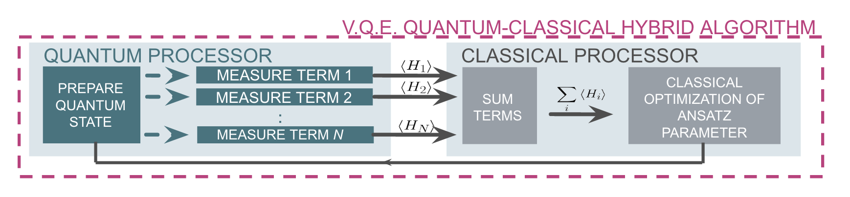
By allowing variational freedom in the \( \beta \) and \( \gamma \) angles QAOA finds the optimal path for a fixed number of steps. Once optimal angles are determined by the classical optimization loop one can read off the distribution by many preparations of the state with \(\beta, \gamma\) and sampling.
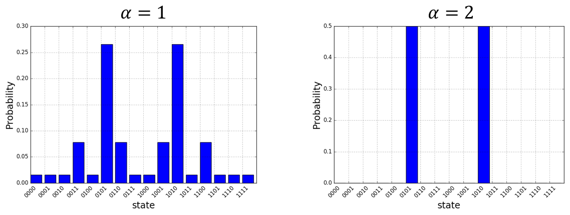
The probability distributions above are for the four ring graph discussed earlier. As expected the approximate evolution becomes more accurate as the number of steps (\(\alpha\)) is increased. For this simple model \(\alpha = 2\) is sufficient to find the two degnerate cuts of the four ring graph.
Source Code Docs
Here you can find documentation for the different submodules in pyQAOA.
grove.pyqaoa.qaoa
-
class
grove.pyqaoa.qaoa.QAOA(qvm, qubits, steps=1, init_betas=None, init_gammas=None, cost_ham=None, ref_ham=None, driver_ref=None, minimizer=None, minimizer_args=None, minimizer_kwargs=None, rand_seed=None, vqe_options=None, store_basis=False)¶ Bases:
objectQAOA object.
Contains all information for running the QAOA algorthm to find the ground state of the list of cost clauses.
N.B. This only works if all the terms in the cost Hamiltonian commute with each other.
Parameters: - qvm – (Connection) The qvm connection to use for the algorithm.
- qubits – (list of ints) The number of qubits to use for the algorithm.
- steps – (int) The number of mixing and cost function steps to use. Default=1.
- init_betas – (list) Initial values for the beta parameters on the mixing terms. Default=None.
- init_gammas – (list) Initial values for the gamma parameters on the cost function. Default=None.
- cost_ham – list of clauses in the cost function. Must be PauliSum objects
- ref_ham – list of clauses in the mixer function. Must be PauliSum objects
- driver_ref – (pyQuil.quil.Program()) object to define state prep for the starting state of the QAOA algorithm. Defaults to tensor product of |+> states.
- rand_seed – integer random seed for initial betas and gammas guess.
- minimizer – (Optional) Minimization function to pass to the Variational-Quantum-Eigensolver method
- minimizer_kwargs – (Optional) (dict) of optional arguments to pass to the minimizer. Default={}.
- minimizer_args – (Optional) (list) of additional arguments to pass to the minimizer. Default=[].
- minimizer_args – (Optional) (list) of additional arguments to pass to the minimizer. Default=[].
- vqe_options – (optinal) arguents for VQE run.
- store_basis – (optional) boolean flag for storing basis states. Default=False.
-
get_angles()¶ Finds optimal angles with the quantum variational eigensolver method.
Stored VQE result
Returns: ([list], [list]) A tuple of the beta angles and the gamma angles for the optimal solution.
-
get_parameterized_program()¶ Return a function that accepts parameters and returns a new Quil program.
Returns: a function
-
get_string(betas, gammas, samples=100)¶ Compute the most probable string.
The method assumes you have passed init_betas and init_gammas with your pre-computed angles or you have run the VQE loop to determine the angles. If you have not done this you will be returning the output for a random set of angles.
Parameters: - betas – List of beta angles
- gammas – List of gamma angles
- samples – (int, Optional) number of samples to get back from the QVM.
Returns: tuple representing the bitstring, Counter object from collections holding all output bitstrings and their frequency.
-
probabilities(angles)¶ Computes the probability of each state given a particular set of angles.
Parameters: angles – [list] A concatenated list of angles [betas]+[gammas] Returns: [list] The probabilities of each outcome given those angles.
grove.pyqaoa.maxcut_qaoa
Finding a maximum cut by QAOA.
-
grove.pyqaoa.maxcut_qaoa.maxcut_qaoa(graph, steps=1, rand_seed=None, connection=None, samples=None, initial_beta=None, initial_gamma=None, minimizer_kwargs=None, vqe_option=None)¶ Max cut set up method
Parameters: - graph – Graph definition. Either networkx or list of tuples
- steps – (Optional. Default=1) Trotterization order for the QAOA algorithm.
- rand_seed – (Optional. Default=None) random seed when beta and gamma angles are not provided.
- connection – (Optional) connection to the QVM. Default is None.
- samples – (Optional. Default=None) VQE option. Number of samples (circuit preparation and measurement) to use in operator averaging.
- initial_beta – (Optional. Default=None) Initial guess for beta parameters.
- initial_gamma – (Optional. Default=None) Initial guess for gamma parameters.
- minimizer_kwargs – (Optional. Default=None). Minimizer optional arguments. If None set to
{'method': 'Nelder-Mead', 'options': {'ftol': 1.0e-2, 'xtol': 1.0e-2, 'disp': False} - vqe_option – (Optional. Default=None). VQE optional arguments. If None set to
vqe_option = {'disp': print_fun, 'return_all': True, 'samples': samples}
-
grove.pyqaoa.maxcut_qaoa.print_fun(x)
grove.pyqaoa.numpartition_qaoa
-
grove.pyqaoa.numpartition_qaoa.numpart_qaoa(asset_list, A=1.0, minimizer_kwargs=None, steps=1)¶ generate number partition driver and cost functions
Parameters: - asset_list – list to binary parition
- A – (float) optional constant for level separation. Default=1.
- minimizer_kwargs – Arguments for the QAOA minimizer
- steps – (int) number of steps approximating the solution.